Modeling Radio Pulsar Selection Effects

Introduction

Double neutron star (DNS) systems – or generally, binaries containing a neutron star and another compact object – are thought to form from the separate evolution of two massive stars in a binary pair. Each star undergoes its supernova explosion, and if both remnants remain gravitationally bound, the outcome can be a neutron star–white dwarf binary, a neutron star–black hole binary, or a double neutron star binary (Chattopadhyay et al. 2020). However, this sequential evolution does not guarantee a surviving binary; one of the supernovae can impart a natal kick strong enough to unbind the system or even cause the two stellar remnants to merge into a single object.
If a binary does remain intact through two supernova events, detecting and measuring the neutron star(s) in such a system is considerably more challenging than for an isolated neutron star. The presence of orbital motion can Doppler-shift and modulate the observed pulsar signal, complicating both detection and parameter estimation. These difficulties in discovering and timing DNS systems are well documented – for example, Bagchi et al. (2013) details the challenges of detecting pulsars in eccentric binaries, and Section 3.9 of Lyne and Grahm-Smith (2012) discusses how binary dynamics can hinder pulsar observations.
A rapidly rotating, highly magnetized neutron star is observed as a pulsar, which emits beams of electromagnetic radiation from its magnetic poles. As the star spins, these beams sweep across the sky; if one of the beams crosses Earth’s line of sight, telescopes record a regular series of pulses. An isolated pulsar typically exhibits extremely stable pulse arrival times, with pulse periods on the order of a few seconds or less. This remarkable regularity allows pulsars to be identified in survey data with high confidence, as genuine pulsar signals appear as strictly periodic flashes separated by a constant interval.
Large pulsar surveys rely on the precision of this periodic timing to distinguish real pulsar signals from random noise. In practice, search algorithms look for strictly periodic sequences of pulses. However, when a pulsar resides in a binary system, its pulse timing is periodically perturbed by the orbital motion. Even slight deviations from perfect periodicity, caused by the pulsar’s changing line-of-sight velocity in a binary, can prevent standard search pipelines from classifying the signal as a pulsar. This selection effect means that some pulsars in binaries may be overlooked in survey data (see Section 3.9 of Lyne and Grahm-Smith 2012 for an indepth discussion).
To assess potential biases in pulsar observations, we calculate the selection effects introduced by the survey for a given pulsar. These calculations account for a variety of factors that can diminish or distort a pulsar’s signal, including propagation through the interstellar medium (e.g. dispersion and scattering by free electrons), receiver noise, and other instrumental or environ- mental effects. In the case of a pulsar in a binary system, we also account for modulation due to orbital dynamics, for example, changes in pulse arrival times caused by the binary motion, which may be exacerbated if the orbit is eccentric or if the companion’s gravity alters the spindown behavior of the pulsar. By modeling these effects, we can infer which pulsars might be missed by a given survey and correct for biases in the measured properties (period, flux, distance, etc.) of those that are detected. Accounting for selection effects in this way allows for a more accurate determination of pulsar intrinsic param- eters. This is crucial because pulsars serve as precise astrophysical tools in many areas (from testing general relativity to probing the interstellar medium), and un- corrected biases could significantly skew any scientific results derived from pulsar data.

Calculating Selection Effects

In this work, we test our selection-effects pipeline – a modernized version of the psrEvolve code (Oslowski et al. 2011) – using a generated population of pulsars. We create a population of binary pulsar systems within a given set of restrictions for their parameters. Given the characteristics of a representative pulsar survey, we then compute the selection effects for each pulsar in our population to evaluate which systems would be detectable and how their observed parameters might be biased by survey sensitivity limits and observational systematics.
To evaluate the ability of a survey to detect a pulsar in a single star or binary system, we calculate four types of selection effects. These include the minimum observable luminosity, the beaming fraction, pulsar death lines, and Bagchi correction. For each selection effect (except the pulsar beaming fraction) it is determined if the pulsar is detected or not. By sorting out all of the non-detections and compiling these effects, we investigate the population of detectable pulsars.
However, to accurately determine the likelihood of a survey detecting the pulsar, we need to consider the fraction of the sky covered by its beam. This is the beaming fraction.
In general, a larger beam width makes detecting the pulsar easier since the survey is more likely to cover an area of the sky that overlaps with the beam. These calculations are applied to each neutron star, whether in isolation or in a binary system.

Results

In both the Python and psrEvolve code (Oslowski et al. 2011) the radiometer equation is implemented first. This is the only selection effect implemented in psrEvolve, so to compare the performance of the Python code to those of psrEvolve, we must only consider this effect. When we calculate all of the resulting selection effects, we used parameters from the SKA survey (Shao et al. 2015). To visually check the distribution of detections returned by python against those given by psrEvolve, we plot P-Pdot diagrams. The P-Pdot diagram illustrates where a pulsar is in it’s life by relating its rotational period (P) to the change in its rotational period (Pdot). We plot the P-Pdot diagram of detections and non-detections for the results of both the psrEvovle and Python code only considering the radiometer equation. By comparing the distribution of ”detected” pulsars we can get an idea of how well the python pipeline is reproducing the results from psrEvolve. In the following figure we removed all the pul- sars which fall below the theoretical death lines given by Chattopadhyay et al. (2020) and Rudak and Ritter (1994). We are not considering the radio efficiency parameters yet. We see that while the distribution of non-detections does not match up well, the overall distribution of detections is good. It can also be observed that the Python pipeline produces fewer non-detections than the psrEvolve code. This is due to a bug in psrEvolve which caused the effective pulse width to be a much higher value and held it constant. Due to the effective pulse width dependence on period, this should not be the case. This is resolved in the Python code and gives it a higher detection rate because the threshold for detectability is lower.

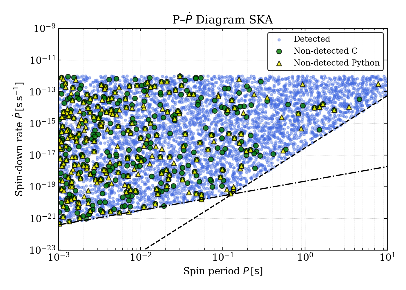Figure 1. Pulsar spin period against spin down period. The distribution of non-detections are marked for both the Python and psrEvolve (Oslowski et al. 2011) outputs. We cut off everything below the theoretical death lines in Chat- topadhyay et al. (2020).
We statistically check the accuracy of the output from python using the KS test. This test measures how sim- ilar the underlying distribution of two samples are and returns the result as a p value. A p value close to 1 means that the two test samples follow a very similar distribution. A p value close to 0 means that the distri- bution of the samples are not significantly similar. We want a p value close to 1 since we need the distribution of detected values by the python pipeline to be very sim- ilar to the detected values returned by psrEvolve. We found a p-value for the SKA survey of 0.981 which means that the Python pipeline reproduces the underlying dis- tribution the C results very well when only using the radiometer equation for selection effects (Figure 3).

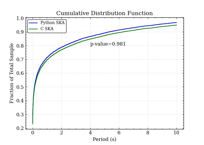Figure 2. Cumulative distribution of detections returned by the Python pipeline compared to the detections returned by the C pipeline. In both of these, the only selection effect that is considered is the radiometer equation.
The second effect that we consider are the death lines of the pulsars. These death lines remove the ”dead” pulsars which are no longer emitting strong radio signals and can therefore not be detected by a survey. The first P-Pdot that we consider removes all of the pulsars which do not have sufficient power in the spin period and magnetic field to accelerate particles and produce the radio emission beams. The second death shown in Figures 1 and 3 marks the theoretical limit where pulsars are unable to produce the election and positron pairs necessary to sustain their radio emissions. However, radio pulsars have been detected beyond the pair production limit. We use a comparison radio effi- ciency factor to the maximum efficiency. This more accurately determines if the pulsar is radio dead by directly determining if it has enough power to sustain radio emissions. As illustrated in Figure 3, this soft cutoff allows some pulsars to fall below the pair production death line, allowing for a more accurate distribution of detections.

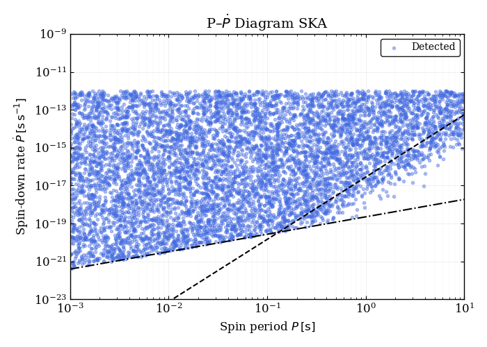Figure 3. Spin period against spin down rate of the generated population of pulsars. In this plot, we only considered the minimum observable luminosity and the death lines.
We have determined that the Python and psrEvolve codes are returning similar results. We now incorporate the effects of the beaming fraction in the detection of pulsars. We weight the detections from the Python code by the beaming fraction to more realistically represent the distribution of detectable pulsars. This distribution is a more realistic example of what we might detect because the pulsars which have shorter spin periods are easier to detect than those with longer spin periods. The shorter the spin period, the more likely it is for the pulsar to be detected by the survey because the pulses are more frequent. This is illustrated in Figure 4. Detections occur frequently at lower spin periods but taper off as the spin periods increase.

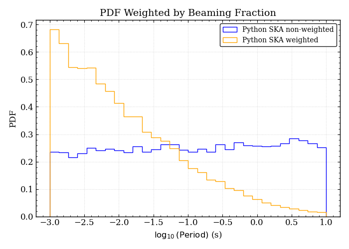Figure 4. Probability density function of both the weighted and unweighted python detections. The weights used are the beaming fractions of the pulsars.
The fourth selection effect that we consider is the Bagchi correction (Bagchi et al. 2013). We investigate how this correction affects the distribution of detections using a fixed orbital period of 3 days for all pulsar binaries in the system. Eccentricity and spin period of the pulsars are allowed to vary. Examining Figure 5, we see that most of the detections are occurring at high eccentricities. These high eccentricities with short orbital periods make the pulsar easier to detect because it does not have as much time to get gravitationally perturbed by it’s more massive companion. In an eccentric orbit the pulsar spends much of the time at aphelion, away from the massive companion. The signal we receive will only occasionally get slightly perturbed when the pulsar sweeps by the massive companion at perihelion. This means much of the time, the pulsar is emitting a steady signal, detectable by a survey.

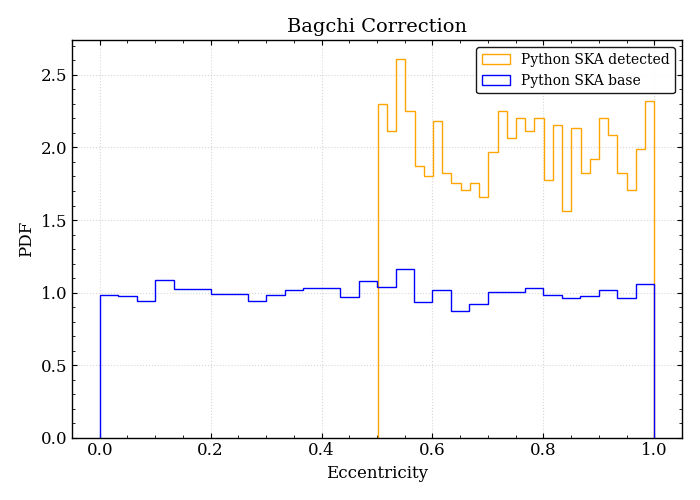Figure 5. Probability density function of the detections returned by the Python pipeline. This data was specifically curated so that each binary system has an orbital period of 3 days.

Summary

We have developed a pipeline to determine selection effects for a population of binary pulsars. This pipeline was created in Python and builds on the psrEvolve pipeline (Oslowski et al. 2011). In the new Python pipeline we include four types of selection effects. These include the minimum detectable luminosity of a pulsar (given by the radiometer equation), the beaming fraction, the pulsar death lines and Bagchi correction.
We run generated data through both pipelines and test the similarity of the results to ensure the Python code is correctly implementing the radiometer equation. We test the similarity of the outputs using K-S testing. The returned p-value indicates that the overall distribution of results from psrEvolve match up well with those from our Python code.
Finally, we test how implementing the other types of selection effects changes the detected population of pulsars.
In future work, we will use POSYDON simulations Fragos et al. (2025) to generate realistic pulsar data with which we will test our selection effects code. The binary pulsar simulations through POSYDON give data in which the pulsar parameters are correlated, unlike the distribution of pulsars used to test the Python pipeline in this work. Applying the selection effects on realistic data will allow us to investigate how they affect a more accurate distribution.
The Python selection effects code is available upon reasonable request to the author.

Acknowledgements

This material is based upon work supported by the National Science Foundation (NSF) under Grant Numbers AST-2149425 and AST-2446392. Any opinions, findings, and conclusions or recommendations expressed in this material are those of the author(s) and do not necessarily reflect the views of the NSF.
This research was supported in part through the computational resources and staff contributions provided for the Quest high performance computing facility at Northwestern University which is jointly supported by the Office of the Provost, the Office for Research, and Northwestern University Information Technology. Thank you to Dr. Debatri Chattopadhyay and Dr. Vicky Kalogera for their mentorship and support.​

Refrences

Bagchi, M., Lorimer, D. R., and Wolfe, S. (2013). On the detectability of eccentric binary pulsars. Monthly Notices of the Royal Astronomical Society, 432(2):1303–1314.
Bovy, J. (2015). galpy: A python library for galactic dynamics. The Astrophysical Journal Supplement Series, 216(2):29. Avaliable at: http://github.com/jobovy/galpy.
Burgay, M., D’Amico, N., Possenti, A., Manchester, R. N., Lyne, A. G., Joshi, B. C., McLaughlin, M. A., Kramer, M., Sarkissian, J. M., Camilo, F., Kalogera, V., Kim, C., and Lorimer, D. R. (2003). An increased estimate of the merger rate of double neutron stars from observations of a highly relativistic system. Nature, 426:531–533.
Chattopadhyay, D., Stevenson, S., Hurley, J. R., Bailes, M., and Broekgaarden, F. (2021). Modelling neutron star–black hole binaries: future pulsar surveys and gravitational wave detectors. Monthly Notices of the Royal Astronomical Society, 504(3):3682–3710.
Chattopadhyay, D., Stevenson, S., Hurley, J. R., Rossi, L. J., and Flynn, C. (2020). Modelling double neutron stars: radio and gravitational waves. Monthly Notices of the Royal Astronomical Society, 494(2):1587–1610.
Chen, K. and Ruderman, M. (1993). Pulsar Death Lines and Death Valley. ApJ, 402:264.
Cordes, J. M. and Lazio, T. J. W. (2002). NE2001.I. A New Model for the Galactic Distribution of Free Electrons and its Fluctuations. arXiv e-prints, pages astro–ph/0207156.
Cordes, J. M. and Lazio, T. J. W. (2003). NE2001. II. Using Radio Propagation Data to Construct a Model for the Galactic Distribution of Free Electrons. arXiv e-prints, pages astro–ph/0301598.
Dewey, R. J., Taylor, J. H., Weisberg, J. M., and Stokes, G. H. (1985). A search for low-luminosity pulsars. ApJL, 294:L25–L29.
Fragos, T., Andrews, J. J., Bavera, S. S., Berry, C. P. L., Coughlin, S., Dotter, A., Giri, P., Kalogera, V., Katsaggelos, A., Kovlakas, K., Lalvani, S., Misra, D., Srivastava, P. M., Qin, Y., Rocha, K. A., Roman-Garza, J., Serra, J. G., Stahle, P., Sun, M., Teng, X., Trajcevski, G., Hai Tran, N., Xing, Z., Zapartas, E., and Zevin, M. (2025). POSYDON: A General-Purpose Population Synthesis Code with Detailed Binary-Evolution Simulations.
Lattimer, J. M. and Schutz, B. F. (2005). Constraining the equation of state with moment of inertia measurements. The Astrophysical Journal, 629(2):979.
Lorimer, D. and Kramer, M. (2005). Handbook of Pulsar Astronomy. Cambridge University Press.
Lyne, A. and Grahm-Smith, F. (2012). Pulsar Astronomy. Cambridge University Press, 4th edition.
Medin, Z. and Lai, D. (2010). Pair cascades in the magnetospheres of strongly magnetized neutron stars. Monthly Notices of the Royal Astronomical Society, 406(2):1379–1404.
Ostriker, J. P. and Gunn, J. E. (1969). On the Nature of Pulsars. I. Theory. ApJ, 157:1395.
Oslowski, S., Bulik, T., Gondek-Rosi´nska, D., and Belczy´nski, K. (2011). Population synthesis of double neutron stars. Monthly Notices of the Royal Astronomical Society, 413(1):461–479.
Pacini, F. (1967). Energy Emission from a Neutron Star. Nature, 216(5115):567–568.
Price, D. C., Flynn, C., and Deller, A. (2021). A comparison of Galactic electron density models using PyGEDM. PASA, 38:e038.
Raithel, C. A., ¨Ozel, F., and Psaltis, D. (2016). Model-independent inference of neutron star radii from moment of inertia measurements. Phys. Rev. C, 93:032801.
Rudak, B. and Ritter, H. (1994). The line of death, the line of birth. Monthly Notices of the Royal Astronomical Society, 267(3):513–517.
Shao, L., Stairs, I., Antoniadis, J., Deller, A., Freire, P., Hessels, J., Janssen, G., Kramer, M., Kunz, J., Laemmerzahl, C., Perlick, V., Possenti, A., Ransom, S., Stappers, B., and van Straten, W. (2015). Testing Gravity with Pulsars in the SKA Era. PoS, AASKA14:042.
Spiewak, R. (2020). skytempy. Accessed on: July 21, 2025. Szary, A., Zhang, B., Melikidze, G. I., Gil, J., and Xu, R.-X. (2014). Radio efficiency of pulsars. The Astrophysical Journal, 784(1):59.
Tauris, T. M. and Manchester, R. N. (1998). On the evolution of pulsar beams. Monthly Notices of the Royal Astronomical Society, 298(3):625–636.
Virtanen, P., Gommers, R., Oliphant, T. E., Haberland, M., Reddy, T., Cournapeau, D., Burovski, E., Peterson, P., Weckesser, W., Bright, J., van der Walt, S. J., Brett, M., Wilson, J., Millman, K. J., Mayorov, N., Nelson, A. R. J., Jones, E., Kern, R., Larson, E., Carey, C. J., Polat, ˙I., Feng, Y., Moore, E. W., VanderPlas, J., Laxalde, D., Perktold, J., Cimrman, R., Henriksen, I., Quintero, E. A., Harris, C. R., Archibald, A. M., Ribeiro, A. H., Pedregosa, F., van Mulbregt, P., and SciPy 1.0 Contributors (2020). SciPy 1.0: Fundamental Algorithms for Scientific Computing in Python. Nature Methods, 17:261–272.
Yamasaki, S. and Totani, T. (2020). The Galactic Halo Contribution to the Dispersion Measure of Extragalactic Fast Radio Bursts. ApJ, 888(2):105.
Yao, J. M., Manchester, R. N., and Wang, N. (2017). A New Electron-density Model for Estimation of Pulsar and FRB Distances. ApJ, 835(1):29.
Young, M. D., Manchester, R. N., and Johnston, S. (1999). A radio pulsar with an 8.5-second period that challenges emission models. Nature, 400(6747):848–849